What is VVC (Versatile Video Coding)? Overview and Comparison with HEVC

In the evolving world of video compression, several new codecs were announced by the MPEG in 2020, such as VVC (Versatile Video Coding), EVC (Essential Video Coding), and LCEVC (Low Complexity Enhancement Video Coding). These codecs have different requirements and satisfy different use-cases, such as efficiently compressing 4K, 8K, or no-royalties (Baseline EVC).

In this architectural overview article, we take a look at the Versatile Video Coding or VVC codec from MPEG and understand its requirements, timeline, and some of the innovative features that make it a video codec to look out for!

History, Requirements, and Timeline of VVC

In October 2015, MPEG and VCEG formed the Joint Video Exploration Team (JVET) tasked with assessing the available compression technologies and exploring the requirements for a next-generation video compression standard. The standardization of VVC began in 2018. 

The main requirements for the new standard were as follows:

• provide algorithms with 30% to 50% better compression compared to the existing HEVC standard at the same quality of experience, with support for lossless and subjectively lossless compression
• support 4K to 16K resolutions as well as VR 360° video
• support the YCbCr color space with 4:4:4, 4:2:2, and 4:2:0 quantization
• 8 bit to 16 bit per component color depth
• BT.2100 and 16+-step High Dynamic Range (HDR)
• auxiliary channels such as depth channel, alpha channel, etc.
• variable and fractional frame rate from 0 to 120 Hz
• scalable coding with temporal (frame rate change) and spatial (resolution change) scalability
• SNR, stereo/multiview coding, panoramic formats, and still image coding.

An up-to-tenfold increase in encoding complexity and twofold increase in decoding complexity was expected compared to HEVC.

The VVC compression standard also known as H.266, ISO/IEC 23090-3, MPEG-I Part 3, and Future Video Coding (FVC) was finalized on July 6, 2020.

This article discusses the most interesting video encoding technologies that have become part of the VVC standard.

Let’s start by looking at VVC’s Coding Structure in the next section.

VVC’s Coding Structure

Slices, Tiles, Subpictures

In VVC, the CTU (coding tree unit) size has increased from 64х64 to 128х128 pixels compared to HEVC. The tiles, slices, and subpictures are now logically separated in the bitstream. Each video frame is split into a regular grid of blocks. VVC implementations can combine several blocks into logical areas defined as tiles, slices, and subpictures.

These methods are already known from earlier codecs, but VVC employs a new way to combine them. The key feature of those areas is that they are logically separated in the bitstream and offer diverse options such as –

• The encoder and decoder can implement concurrent processing.
• The decoder may elect only to decode the areas of the video that it needs (one possible application is transmitting panoramic video, where the user may see only parts of the full video)
• The bitstream can be encoded to extract a part of the video stream on the fly without re-encoding.

Block Splitting in VVC

In HEVC, there was a single tree structure that allowed the splitting of each square block into 4 square sub-blocks recursively. However, VVC now offers several possible splitting operations within a multi-tree structure.

• The first split is into a quaternary tree, as in HEVC.
• Then each block can be split horizontally and vertically into 2 (BT split) or 3 (TT split) parts.

This step is again performed recursively so that each rectangular block can be further split into 2 or 3 parts horizontally or vertically. Such an approach enables much better adaptation of the encoder to the input and considerably increases the complexity of video coding.

Furthermore, the luma (luminance coding) and chroma (chromaticity coding) blocks can be different, forming a double-tree structure. In other words, the chroma samples can have a coding-tree structure that is independent of the luma samples within the same CTU. This makes it possible to use larger coding blocks for chroma samples than for luma samples.

Spatial Block Prediction in VVC

We first look at the spatial prediction (intra) options in VVC and then move on to the inter prediction.

For intra-prediction, the existing Planar, DC, PCM, and Angular Prediction modes are still available. The number of directions for Angular Prediction has been increased from 33 (in HEVC) to 65.

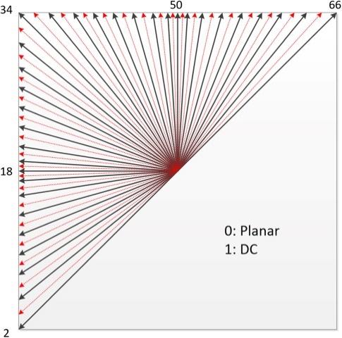
Wide Angle Intra Prediction

Since prediction blocks may be non-square in VVC, traditional modes are adaptively replaced by wide-angle directions (Wide Angle Intra Prediction). Therefore, VVC implementations can use more reference pixels for prediction. Essentially, this widens the prediction direction angles to values that exceed the normal 45° and –135°.

Position-Dependent Prediction Combination

A new Position-dependent prediction combination mode has been added, in which directional interpolation is possible. It combines the spatial (Intra) prediction with a position-dependent weighting of some primary and reference samples.

Cross-Component Prediction

Furthermore, in many cases, the luma and chroma components carry very similar information, therefore a new prediction mode called Cross-component Prediction was added for those cases. In this mode, a method is used that directly predicts chroma components from a reconstructed luma block using a linear combination of reconstructed pixels with two parameters, a factor, and an offset, where the factors are calculated from the intra reference pixels. The block is also scaled if necessary.

Multi Reference Line Prediction

It is now possible in VVC to make a prediction using two lines that are not directly adjacent to the current block; this is called Multi Reference Line Prediction.

Inter-frame prediction

The basic concepts of uni-directional and bi-directional motion compensation from one or two reference pictures are mostly unchanged. However, there are some new tools that have not been used in a video coding standard before.

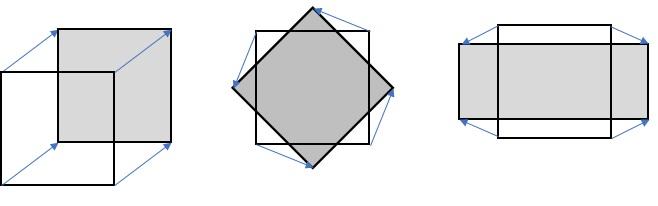
Affine Motion Estimation Model in VVC

The conventional motion compensation represents two-dimensional planar motion. This kind of motion is rarely encountered in actual videos, however, because objects move more freely and/or change their shape. For these cases, the Affine motion model was implemented in VVC that uses two or three vectors to enable motion with four or six degrees of freedom.

The maximum luma motion vector precision increases from 1/4 to 1/16 of a pixel, and the corresponding chroma motion vector precision increases from 1/16 to 1/32 of a pixel.

You can now use Adaptive motion vector resolution for encoding. This helps reduce coding costs for large values of MV, which is especially relevant for high resolutions (4K and higher).

Overlapped Block Motion Compensation & BDOF in VVC

A method for compensating the motion of overlapping blocks is now available. This method, called Overlapped Block Motion Compensation, overlaps the edges of the adjacent blocks and then smooths them to avoid sharp transitions that usually occur with inter-prediction. 

If the block uses bi-directional prediction, the new BDOF (Bi-directional optical flow) method can be used to refine the motion of the prediction block. This algorithm does not require decoder signaling and provides 2% to 6% bitrate savings.

Decoder-Side Motion Vector Refinement

Decoder side motion vector refinement makes it possible to refine motion vectors in the decoder without transmitting additional motion data. This process consists of three stages. First, a bi-directional prediction is performed, and the data is weighted into a preliminary prediction block. Then a search is performed around the position of the original block with a fixed number of positions. If a better position is found, the original motion vector is updated accordingly. Finally, a new bi-directional prediction is performed with the updated motion vectors to obtain the final prediction.

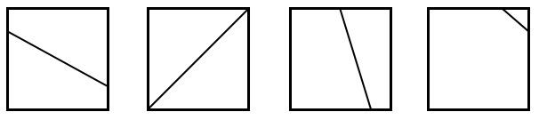
Geometric Partitioning

Rectangular blocks usually do not work well for predicting real video. For more effective prediction, Geometric Partitioning has been added in VVC. This option allows non-horizontal splitting of a block into two parts with separate motion compensation for each one. The current implementation includes 82 different geometric partitioning modes. 

Transforms and quantization

The maximum transform block size has been increased to 64×64 in VVC. These transforms are especially useful when it comes to HD and Ultra-HD content.

Unlike HEVC that only has a single DCT (DCT-II) transform, VVC has 4 separable ones:

• DCT (DCT-VIII) – a type-VIII discrete cosine transform
• DST-VII – a discrete sine transform.

The encoder can select different transforms depending on the prediction mode.

Adaptive Loop Filter

The Adaptive Loop Filter in the VVC standard has the following features:

• a 7×7 diamond filter (13 different coefficients) is used for luma components and a 5х5 diamond filter (7 different coefficients) for chroma components
• each 4х4 luma block is categorized into one of 25 different classes using vertical, horizontal, and two diagonal gradients
• based on the calculated gradients, the filter coefficients can undergo one of three transforms-diagonal reflections, vertical reflection, or rotation-before they are applied.

HEVC vs. VVC Performance Evaluation

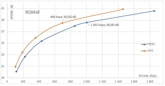
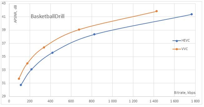
The following graphs show the results of encoding two test sequences using the HEVC HM 16.15 and VVC VTM-12.0 reference encoders. In both cases, the encoding was performed using a standard configuration file (randomaccess.cfg) and equally optimized encoders.

As seen in the graphs (Fig. 1 and Fig. 2), the coding efficiency of VVC exceeds that of the previous standard at all bitrates. Consider the BQMall graph (Fig. 1) and the values obtained in its middle section.

For the HEVC sequence, we obtained a bitrate of 1002 kbps and an APSNR of 38.58 dB. To achieve a similar quality using VVC coding, a bitrate of 696 kbps would be sufficient (at an APSNR of 38.50 dB), yielding bitrate savings of 30%.

The encoding time for the HEVC encoder was about 16 minutes, whereas for VVC it amounted to 2.29 hours, which is 9.3 times longer.

Conclusion

We come to this architectural overview of VVC (Versatile Video Coding). I hope you have a better understanding of this new and upcoming video coding standard, understood its features, and have understood the difference in performance between VVC and HEVC.