Affine Motion Compensated Prediction in VVC

This article will take a closer look at the Affine Motion Compensated Prediction in the VVC (Versatile Video Coding) codec and demonstrate how it works. 

MPEG developed three new video codecs in 2020-2021 – Versatile Video Coding (H.266), Essential Video Coding (EVC MPEG-5 Part 1), and Low Complexity Enhancement Video Coding (LCEVC MPEG-5 Part 2). The VVC codec is considered as a successor to H.265 (HEVC) and has several advanced inter-prediction coding tools used for frame compression.

One of them is Affine Motion Inter-Prediction. In this article we will explore the concepts of affine motion estimation and compensation in the VVC codec with examples and how to understand them using a VQ analyzer.

What is Prediction in Video Codecs?

Prediction modes are basically subdivided into two main types:

• Intra – when pixels are predicted by other pixels of the current frame,
• Inter – when other frames predict the current frame.

Inter Prediction technique uses optical flow, where every pixel on the frame can have a vector from the previous frame. However, signaling every vector uses a considerable amount of data, which is costly. For this reason, an image is split into blocks called prediction units (PU). Every block has only one summarized motion vector (or two in the case of Bi-prediction).

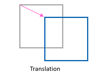
Classical motion compensation works with 2D translations – 2 degrees of freedom (DOF).

It happens when you just copy one rectangular block from one place to another. However, the real world is always a bit more complicated. There is not much stuff that simply moves plainly over the screen, unless it is Super Mario, of course. Objects often rotate, scale, and combine different types of motion. Some of those movements could be presented with Affine Transformations. 

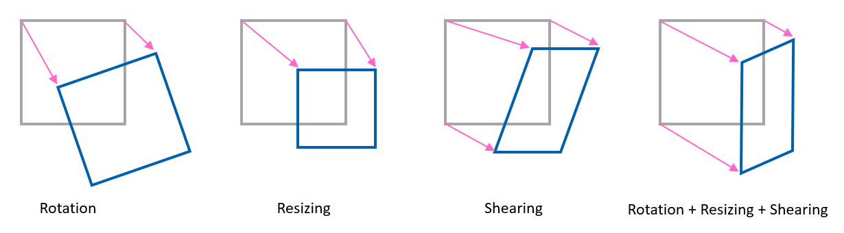
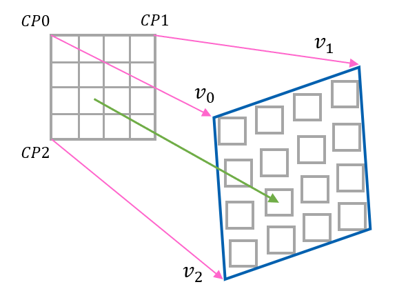
Therefore, the idea of Affine Prediction is to extend the classical translation (2 DOF) to more degrees of freedom. Affine transformation is a geometric transformation that preserves the lines and parallelism. VVC has two models of describing affine motion information: using two control points (4-parameter) or three control point motion vectors (6-parameter):

• Classic prediction: 2D translation
• Affine 4 param: + rotation, scaling
• Affine 6 param: + aspect ratio, shearing

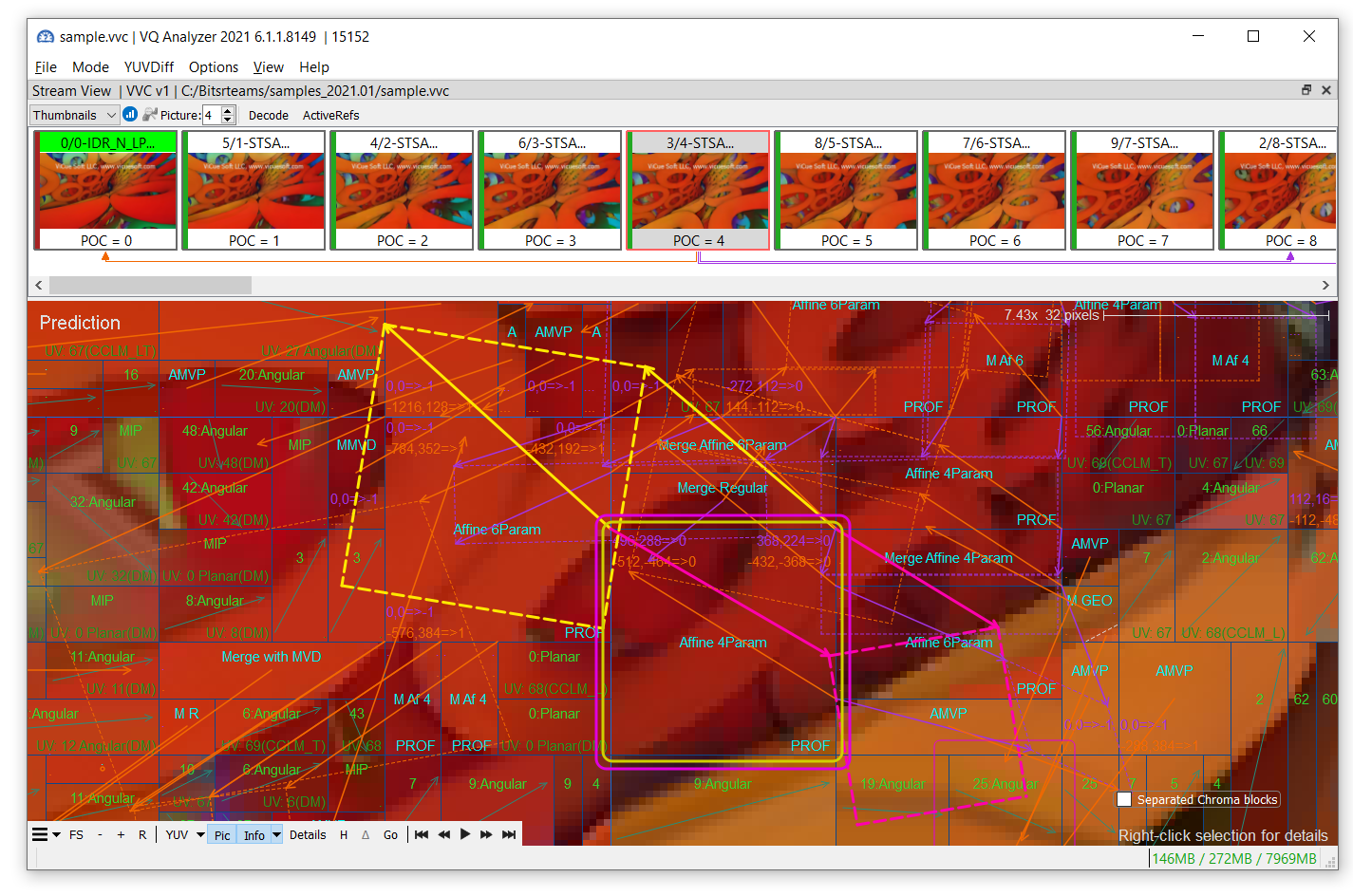
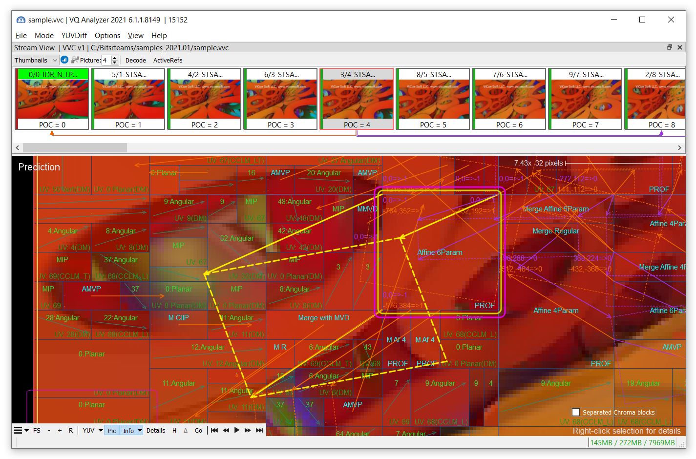
Let us now consider examples of Affine prediction using VQ Analyzer.

Implementation of Affine Motion Estimation in VVC

To lower computation complexity and memory access in hardware implementations, VVC simplifies the affine model that is block-based. Instead of applying vectors for each pixel, the block is divided into 4×4 pixel luma sub-blocks. VVC signals corner motion vectors for CU. Subblock MVs are derived from block control point MVs, according to the equations below, and rounded to 1/16 fraction accuracy. Then translational motion compensation is applied for each sub-block.

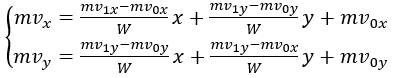
For a 4-parameter affine motion model, the motion vector at sample location (x, y) in a block is derived as:

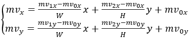
For a 6-parameter affine motion model, the motion vector at sample location (x, y) in a block is derived as:

There are two affine motion prediction modes in VVC:

• affine merge mode,
• and affine AMVP mode.

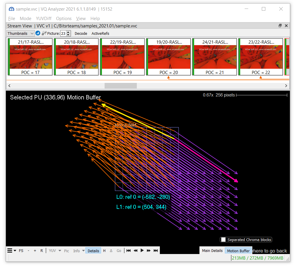
VQ analyzer can display sub-blocks motion vectors in Details View of Motion buffer:

There are two Affine motion prediction modes in VVC:

• Affine merge mode
• Affine AMVP mode

Affine Merge Prediction in VVC

In this mode, motion information of spatial neighbor blocks is used to generate CPMVs for the current CU. There could be up to five candidates. The chosen candidate index is signaled in the stream. Candidates could be:

• Inherited (extrapolated) from neighbors 
• Constructed from translation motion vectors
• Zero motion vectors.

We will now provide examples of all of them. 

Inherited candidates

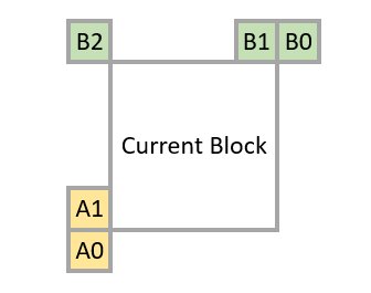
There could be up to 2 inherited MVs; they are obtained from neighbors left-bottom (A0->A1) and right-top (B0->B1->B2), if available.

Constructed candidates

Constructed affine candidates are the combinations of neighbors’ translational motion vectors. They are produced in two steps.     

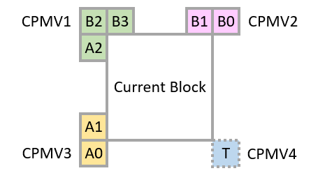
Step 1. Obtain CPMVs vectors from the available neighbors:

• CPMV1 – one from B2->B3->A2
• CPMV2 – one from B1->B0
• CPMV3 – one from A1->A0
• CPMV4 – temporary motion vector prediction, if available

Step 2. Derive combinations:

{CPMV1, CPMV2, CPMV3}, {CPMV1, CPMV2, CPMV4}, {CPMV1, CPMV3, CPMV4},

{CPMV2, CPMV3, CPMV4}, {CPMV1, CPMV2}, {CPMV1, CPMV3}

When the list is not complete after filling with inherited and constructed candidates, zero MVs are inserted at the end of the list.

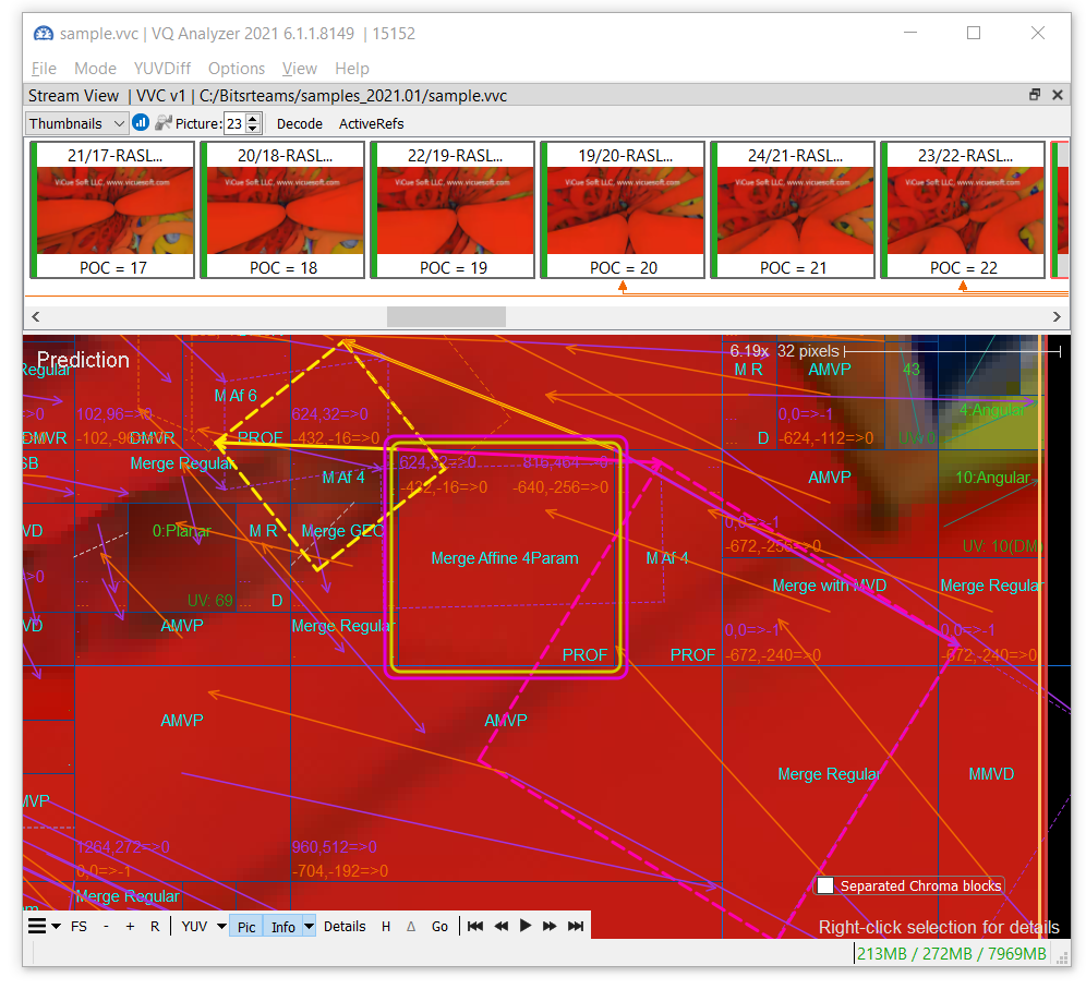
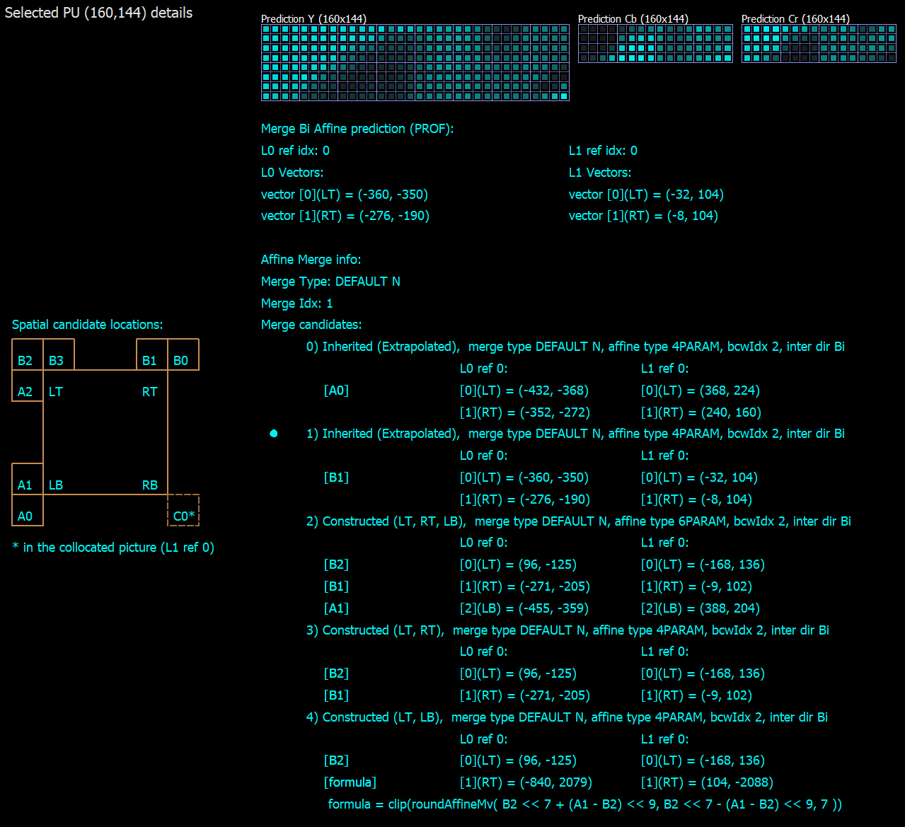
You can view affine block prediction details, including the candidate list in Detail View of VQ Analyzer. Here is an Affine Merge example:

Affine AMVP prediction

In affine AMVP (advanced motion vector prediction) mode, the difference between vectors of current CU and their predictors is added to the bitstream:

CPMV = prediction + difference

Prediction is obtained using the candidate list; it is limited to 2 candidates.

Candidates could be:

• Inherited (extrapolated) from neighbors 
• Constructed from translation motion vectors
• Translational MVs from neighboring CUs
• Zero motion vectors.

The checking order of inherited and constructed affine AMVP candidates is the same as in the Merge mode, but it has an additional check – the candidate must have the same reference picture index. 

Constructed candidates could be {CPMV1, CPMV2} for 4-param mode and {CPMV1, CPMV2, CPMV3} for 6 param mode.

Affine AMVP details and the candidate list also could be accessed in VQ Analyzer Detail View for a selected block:

That is all for today. In this article, we have demonstrated the affine prediction algorithm in VVC.